B-trees: the filing system behind fast databases

A B-tree is a balanced multiway search tree.^[4] In PostgreSQL, internal pages direct searches towards the next level and leaf pages occupy the lowest level.^[1] Multiple keys per node allow a search to discard every branch except the interval that can contain the target.

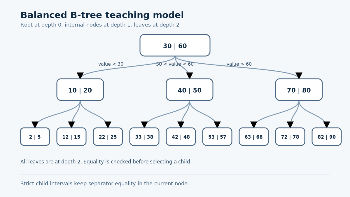
Keys create strict child intervals

In the teaching model, the root stores 30 and 60. Equality is tested in that node. Only unequal values descend: values below 30 use child 0, values strictly between 30 and 60 use child 1, and values above 60 use child 2. Every internal node applies the same convention.

The corrected model has three levels. The root is at depth 0, each internal child is at depth 1, and all nine leaves are at depth 2. The validator checks ordered and unique keys, range bounds, the rule that an internal node with k keys has k + 1 children, and equal leaf depths. These checks describe this executable teaching model rather than every storage detail of a database implementation.

Finding 42, one decision at a time

The search first visits [30, 60]. Since 30 < 42 < 60, it selects child 1. The next node stores [40, 50]. Since 40 < 42 < 50, the search again selects child 1 and reaches the leaf [42, 48]. The other branches are not visited.

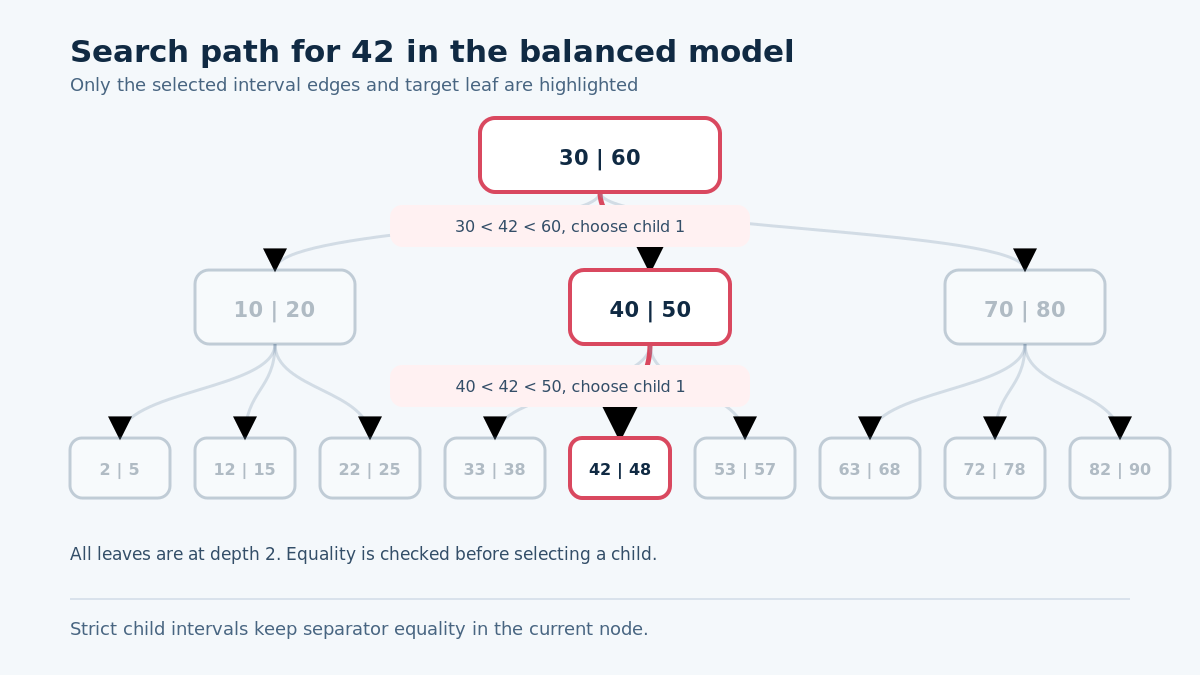
Equality follows a different path. A search for 60 succeeds at the root before any child is selected. A search for the absent key 41 follows the same two middle intervals and stops at [42, 48], the only leaf whose range could contain it.

An executable balanced teaching model

Python documents bisect_right() as returning an insertion position to the right of an existing equal value.^[5] The program checks equality first, so bisect_right() is used only to select the strict child interval.

The following complete Python program builds the corrected tree, validates its structure, and runs successful, separator-equality and absent-key searches. It omits insertion, deletion, page layout, concurrency and recovery, so it is a search model rather than a production B-tree.

from bisect import bisect_right
from dataclasses import dataclass, field
@dataclass
class Node:
    keys: list[int]
    children: list["Node"] = field(default_factory=list)
    @property
    def is_leaf(self) -> bool:
        return not self.children
def validate(root: Node) -> list[int]:
    leaf_depths: list[int] = []
    def visit(node: Node, low: int | None, high: int | None, depth: int) -> None:
        assert node.keys == sorted(node.keys)
        assert len(set(node.keys)) == len(node.keys)
        assert all((low is None or low < key) and (high is None or key < high)
                   for key in node.keys)
        if node.is_leaf:
            leaf_depths.append(depth)
            return
        assert len(node.children) == len(node.keys) + 1
        bounds = [low, *node.keys, high]
        for index, child in enumerate(node.children):
            visit(child, bounds[index], bounds[index + 1], depth + 1)
    visit(root, None, None, 0)
    assert len(set(leaf_depths)) == 1
    return leaf_depths
def search(root: Node, target: int) -> bool:
    node = root
    while True:
        print(f"Visit {node.keys}")
        if target in node.keys:
            print(f"Found {target}")
            return True
        if node.is_leaf:
            print(f"{target} is not in the tree")
            return False
        branch = bisect_right(node.keys, target)
        print(f"Take child {branch}")
        node = node.children[branch]
tree = Node(
    [30, 60],
    [
        Node([10, 20], [Node([2, 5]), Node([12, 15]), Node([22, 25])]),
        Node([40, 50], [Node([33, 38]), Node([42, 48]), Node([53, 57])]),
        Node([70, 80], [Node([63, 68]), Node([72, 78]), Node([82, 90])]),
    ],
)
depths = validate(tree)
print("Leaf depths:", depths)
print("Tree valid:", len(set(depths)) == 1)
for target in (42, 60, 41):
    print(f"\nSearch for {target}:")
    search(tree, target)

Executed with Python 3.13.5, the program produced this exact output:

Leaf depths: [2, 2, 2, 2, 2, 2, 2, 2, 2]
Tree valid: True
Search for 42:
Visit [30, 60]
Take child 1
Visit [40, 50]
Take child 1
Visit [42, 48]
Found 42
Search for 60:
Visit [30, 60]
Found 60
Search for 41:
Visit [30, 60]
Take child 1
Visit [40, 50]
Take child 1
Visit [42, 48]
41 is not in the tree

When a page runs out of room

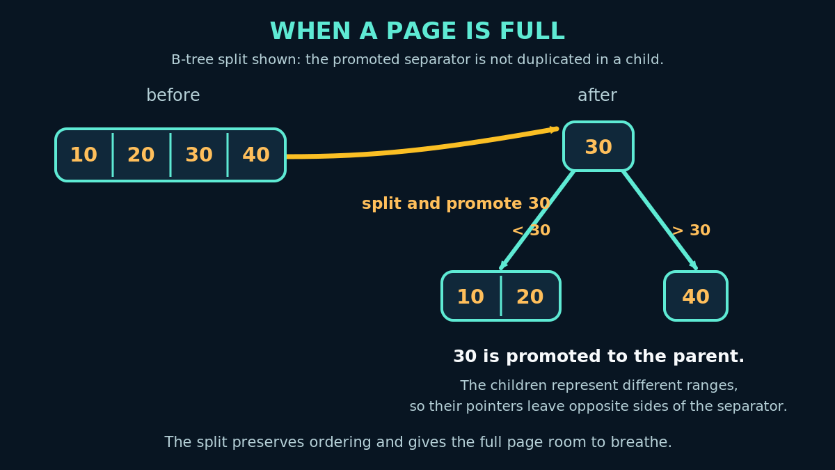
PostgreSQL adds a new leaf page when an existing leaf page cannot accept an incoming tuple. Page splits can cascade upwards, and a root split adds a new level above the previous root.^[1] A valid split preserves the ordering and balance invariants of the tree.

B-tree and B+ tree terminology

A B+ tree uses internal values to guide a search and normally stores record references at the leaf level. Its leaves are commonly linked to support ordered access.^[2] The executable model above instead treats keys in internal nodes as stored keys, so equality with an internal key is resolved in that node. The interval labels and code therefore describe one consistent B-tree teaching convention.

Watching SQLite choose an index

SQLite delegates the choice of an execution method to its query planner. Its documentation describes binary search over an index as a way to locate the relevant subset of rows.^[3] The next program creates 10,000 rows in memory and records the plan descriptions before and after creating an index.

import sqlite3
db = sqlite3.connect(":memory:")
db.execute("CREATE TABLE products (id INTEGER PRIMARY KEY, name TEXT, price REAL)")
db.executemany(
    "INSERT INTO products (name, price) VALUES (?, ?)",
    [(f"Product {n}", n / 10) for n in range(1, 10_001)],
)
query = "SELECT name FROM products WHERE price = 42.0"
print("Before the index:")
print(db.execute(f"EXPLAIN QUERY PLAN {query}").fetchone()[3])
db.execute("CREATE INDEX products_price_idx ON products(price)")
print("After the index:")
print(db.execute(f"EXPLAIN QUERY PLAN {query}").fetchone()[3])
print("Result:", db.execute(query).fetchone()[0])

Executed with the locally recorded Python and SQLite versions, the program produced this exact output:

Before the index:
SCAN products
After the index:
SEARCH products USING INDEX products_price_idx (price=?)
Result: Product 420

The first plan scans products. After products_price_idx is created, the plan reports an index search and returns Product 420. The plan text is evidence for this SQLite build and query; another release may format an equivalent plan differently.

Index costs and query selection

B-tree indexes occupy storage and can require page maintenance when indexed data changes.^[1] Whether a query uses an available index remains a query-planner decision. The appropriate index set therefore depends on observed queries, write workload, data distribution and measured plans.^[3]

Sources

• [1] PostgreSQL, B-Tree Indexes
• [2] University of Cape Town, Database Systems: B-trees and B+ trees
• [3] SQLite, Query Planning
• [4] NIST Dictionary of Algorithms and Data Structures, B-tree
• [5] Python documentation, bisect