Binary search in Python: stop checking every item

Suppose a sorted list contains 20,000 product IDs and must answer 2,000 lookups. A linear search starts at the beginning and advances until it finds the target or passes its possible position. In the worst case it examines every item, so its running time is O(n).^[3]

Binary search uses the sorted order. It checks the middle item and discards the half that cannot contain the target, repeating until it finds the value or the interval is empty. NIST defines the method for sorted arrays and gives its running time as O(log n).^[2] Python’s bisect module supplies insertion-point operations for sorted sequences.^[1]

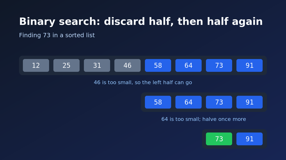
Three stages of binary search narrowing a sorted list from eight values to the target 73 — Half the candidates leave after every comparison. Ruthless, but efficient.

Why halving changes the operation count

A linear membership test on a Python list is O(n), while indexed list access is O(1) on average.^[3] Binary search therefore needs a sequence that is already sorted and supports suitably cheap access to middle elements. For 20,000 items, repeatedly halving the candidate interval requires at most about 15 midpoint decisions in this implementation.

Maintaining order has a separate cost. Python documents insort as O(n) overall because its logarithmic search is dominated by the linear insertion step.^[1] The appropriate data structure therefore depends on both lookup and update patterns.

Reproducible comparison

The complete program below builds a seeded workload, verifies that both methods return the same answers, records seven timing runs and counts the elements or midpoints inspected.

from bisect import bisect_left
from random import Random
from statistics import median
from timeit import repeat
import platform
N = 20_000
Q = 2_000
REPEAT = 7
rng = Random(20260812)
values = list(range(0, N * 2, 2))
targets = [rng.randrange(0, N * 2) for _ in range(Q)]
def linear_search(a, x):
    for i, value in enumerate(a):
        if value >= x:
            return i if value == x else -1
    return -1
def binary_search(a, x):
    i = bisect_left(a, x)
    return i if i != len(a) and a[i] == x else -1
def run(search):
    return [search(values, target) for target in targets]
expected = run(linear_search)
assert run(binary_search) == expected
linear_times = repeat("run(linear_search)", globals=globals(), number=1, repeat=REPEAT)
binary_times = repeat("run(binary_search)", globals=globals(), number=1, repeat=REPEAT)
linear_median = median(linear_times)
binary_median = median(binary_times)
# Count inspected elements for the same workload using transparent Python versions.
def linear_search_counted(a, x):
    checks = 0
    for i, value in enumerate(a):
        checks += 1
        if value >= x:
            return (i if value == x else -1), checks
    return -1, checks
def binary_search_counted(a, x):
    lo, hi, checks = 0, len(a), 0
    while lo < hi:
        mid = (lo + hi) // 2
        checks += 1
        if a[mid] < x:
            lo = mid + 1
        else:
            hi = mid
    found = lo != len(a) and a[lo] == x
    return (lo if found else -1), checks
linear_checks = sum(linear_search_counted(values, x)[1] for x in targets)
binary_checks = sum(binary_search_counted(values, x)[1] for x in targets)
print(f"Python: {platform.python_implementation()} {platform.python_version()}")
print(f"Platform: {platform.platform()}")
print(f"Dataset: {N:,} sorted integers; {Q:,} seeded lookups; {REPEAT} repeats")
print(f"Matches: {sum(i >= 0 for i in expected):,}")
print(f"Linear median: {linear_median:.6f} s")
print(f"bisect median: {binary_median:.6f} s")
print(f"Speed ratio: {linear_median / binary_median:.1f}x")
print(f"Linear inspected elements: {linear_checks:,}")
print(f"Binary comparisons: {binary_checks:,}")
print(f"Comparison ratio: {linear_checks / binary_checks:.1f}x")

Recorded local execution

The artefact was executed on 13 August 2026. The seeded workload produced 1,018 matches, 20,088,518 inspected elements for the linear scan and 28,703 midpoint comparisons for binary search. These deterministic counts match the previously published benchmark. Timing values below are the exact output of this execution and are specific to the reported interpreter, operating system and workload.

Python: CPython 3.13.5
Platform: Linux-6.12.47+rpt-rpi-v8-aarch64-with-glibc2.41
Dataset: 20,000 sorted integers; 2,000 seeded lookups; 7 repeats
Matches: 1,018
Linear median: 2.442080 s
bisect median: 0.002884 s
Speed ratio: 846.7x
Linear inspected elements: 20,088,518
Binary comparisons: 28,703
Comparison ratio: 699.9x

The operation counts explain the direction of the timing result without treating the measured ratio as universal. bisect_left also runs in CPython’s optimised implementation while the baseline loop executes Python bytecode, so the stopwatch comparison measures both algorithm choice and implementation.^[1]

Conditional selection criteria

Binary search is applicable when the data is sorted, midpoint access is sufficiently cheap, and enough searches are expected to justify the cost of obtaining or preserving that order.^[1]^[2] It also supports boundary queries such as finding an insertion point or the first value at or after a threshold.^[1]

For a single lookup in unsorted data, one scan avoids the separate sorting cost. For exact key membership where ordering and boundary positions are not required, Python’s documentation notes that dictionaries are more performant than bisection for locating specific values, subject to memory, key-hashability and workload constraints.^[1]^[3] For small collections, measurement on the actual workload is needed because constant costs are not described by Big O notation.