Dijkstra in Python: replace the full scan with a heap

Finding a shortest route in a weighted graph is easy to describe and surprisingly easy to make slower than it needs to be. The algorithm must repeatedly choose the unsettled node with the smallest known distance, then use that node to improve its neighbours. A basic implementation scans every node to make that choice, including nodes that are already settled or still unreachable.^[3]^[4]

A priority queue changes that part of the job. Instead of asking the whole graph which candidate is smallest, the implementation keeps promising candidates in a min-heap and takes the smallest entry from the top.^[1]^[4] The graph work is still there. The wasted search for the next node is what gets trimmed.

The problem is finding the next node

Dijkstra’s algorithm solves a single-source shortest-path problem when edge weights are non-negative.^[4]^[5] A weight might represent distance, travel time or a monetary cost. The algorithm starts with distance zero for the source and infinity for every other node. Each time it selects a node, it relaxes an outgoing edge: if reaching a neighbour through the selected node is cheaper than the current estimate, the estimate is replaced.^[4]^[5]

The relaxation step is not the expensive-looking part in a small Python program. The awkward bit is selecting the next node. A straightforward version loops over the complete distance array on every round. With V nodes, that selection costs O(V) per round and reaches O(V²) overall, plus the cost of examining edges.^[5]

The heap version stores pairs such as (distance, node). Python’s heapq module implements a min-heap in an ordinary list, with the smallest item at index zero; pushing and popping maintain the heap invariant.^[1] Python’s interface does not expose the same decrease-key operation used in many textbook presentations, so the program pushes a new pair when a distance improves and ignores an older pair when it later comes out of the heap.

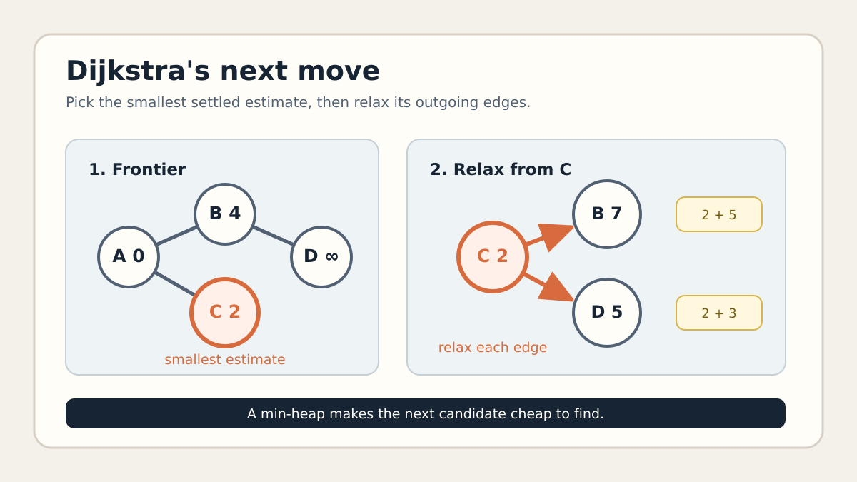
Diagram showing Dijkstra selecting node C with distance 2 and relaxing edges to update B and D — Dijkstra picks the smallest known estimate, then gives its neighbours a chance to improve.

That stale-entry check is a small implementation detail with a large correctness role. A node may appear several times in the heap, but only the pair whose distance matches the current best estimate is allowed to relax edges. The code below uses that approach and computes distances from node 0 to every reachable node.

A complete comparison

The following program contains both versions. It generates the same deterministic positive-weight graph for each case, checks that the distance arrays match, counts the main operations and records timing and traced Python allocations. The graph is directed, every node is reachable through a chain, and extra edges are generated from fixed seeds.

The timing uses five timeit.repeat repeats with three executions per repeat, reporting the best repeat. Python’s documentation recommends repeated measurements because other processes can disturb wall-clock timings, and notes that timeit disables garbage collection by default.^[2] The memory number is the peak allocation seen by tracemalloc during one run, not the resident memory of the whole process.

from __future__ import annotations
import json
import platform
import random
import sys
import timeit
import tracemalloc
from heapq import heappop, heappush
Graph = list[list[tuple[int, int]]]
def make_graph(node_count: int, edge_count: int, seed: int) -> Graph:
    """Build a deterministic, reachable directed graph with positive weights."""
    rng = random.Random(seed)
    graph: Graph = [[] for _ in range(node_count)]
    used: set[tuple[int, int]] = set()
    for node in range(node_count - 1):
        weight = rng.randint(1, 20)
        graph[node].append((node + 1, weight))
        used.add((node, node + 1))
    while len(used) < edge_count:
        start = rng.randrange(node_count)
        finish = rng.randrange(node_count)
        if start == finish or (start, finish) in used:
            continue
        graph[start].append((finish, rng.randint(1, 20)))
        used.add((start, finish))
    return graph
def dijkstra_scan(graph: Graph, source: int) -> tuple[list[float], dict[str, int]]:
    """Baseline: scan every unvisited node to find the next smallest distance."""
    infinity = float("inf")
    distances = [infinity] * len(graph)
    visited = [False] * len(graph)
    distances = 0
    scans = 0
    relax_checks = 0
    for _ in graph:
        next_node = -1
        next_distance = infinity
        for node, distance in enumerate(distances):
            scans += 1
            if not visited[node] and distance < next_distance:
                next_node = node
                next_distance = distance
        if next_node == -1:
            break
        visited[next_node] = True
        for neighbour, weight in graph[next_node]:
            relax_checks += 1
            candidate = next_distance + weight
            if candidate < distances[neighbour]:
                distances[neighbour] = candidate
    return distances, {"scans": scans, "relax_checks": relax_checks}
def dijkstra_heap(graph: Graph, source: int) -> tuple[list[float], dict[str, int]]:
    """Optimised version: heapq stores candidate distances; stale entries are skipped."""
    infinity = float("inf")
    distances = [infinity] * len(graph)
    distances = 0
    pending = [(0, source)]
    pushes = 1
    pops = 0
    stale_pops = 0
    relax_checks = 0
    while pending:
        distance, node = heappop(pending)
        pops += 1
        if distance != distances[node]:
            stale_pops += 1
            continue
        for neighbour, weight in graph[node]:
            relax_checks += 1
            candidate = distance + weight
            if candidate < distances[neighbour]:
                distances[neighbour] = candidate
                heappush(pending, (candidate, neighbour))
                pushes += 1
    return distances, {
        "pushes": pushes,
        "pops": pops,
        "stale_pops": stale_pops,
        "relax_checks": relax_checks,
    }
def measure(function, graph: Graph) -> dict[str, object]:
    """Return repeat timings and peak allocations for one fixed graph."""
    timings = timeit.repeat(lambda: function(graph, 0), repeat=5, number=3)
    tracemalloc.start()
    distances, operations = function(graph, 0)
    _, peak_bytes = tracemalloc.get_traced_memory()
    tracemalloc.stop()
    return {
        "best_seconds_for_three_runs": min(timings),
        "repeat_seconds_for_three_runs": timings,
        "peak_traced_bytes": peak_bytes,
        "reachable_nodes": sum(distance < float("inf") for distance in distances),
        "operations": operations,
    }
def main() -> None:
    cases = {
        "sparse": make_graph(node_count=800, edge_count=2_400, seed=20260824),
        "denser": make_graph(node_count=600, edge_count=36_000, seed=20260825),
    }
    results: dict[str, object] = {
        "environment": {
            "python": sys.version.split()[0],
            "implementation": platform.python_implementation(),
            "platform": platform.platform(),
        },
        "method": {
            "timing": "timeit.repeat(repeat=5, number=3), best repeat reported",
            "memory": "one tracemalloc run, peak traced Python allocations",
            "weights": "positive integers from 1 to 20",
        },
        "cases": {},
    }
    for name, graph in cases.items():
        scan = measure(dijkstra_scan, graph)
        heap = measure(dijkstra_heap, graph)
        scan_distances, _ = dijkstra_scan(graph, 0)
        heap_distances, _ = dijkstra_heap(graph, 0)
        if scan_distances != heap_distances:
            raise AssertionError(f"distance mismatch in {name}")
        results["cases"][name] = {
            "nodes": len(graph),
            "edges": sum(len(edges) for edges in graph),
            "scan": scan,
            "heap": heap,
            "same_distances": True,
            "relative_best_time_scan_divided_by_heap": (
                scan["best_seconds_for_three_runs"]
                / heap["best_seconds_for_three_runs"]
            ),
        }
    print(json.dumps(results, indent=2))
if __name__ == "__main__":
    main()

The captured output below came from executing that exact file on CPython 3.13.5 on a Raspberry Pi running Linux 6.12.47, using the two fixed graphs described in the source.

{
  "environment": {
    "python": "3.13.5",
    "implementation": "CPython",
    "platform": "Linux-6.12.47+rpt-rpi-v8-aarch64-with-glibc2.41"
  },
  "method": {
    "timing": "timeit.repeat(repeat=5, number=3), best repeat reported",
    "memory": "one tracemalloc run, peak traced Python allocations",
    "weights": "positive integers from 1 to 20"
  },
  "cases": {
    "sparse": {
      "nodes": 800,
      "edges": 2400,
      "scan": {
        "best_seconds_for_three_runs": 0.41016848298022524,
        "repeat_seconds_for_three_runs": [
          0.4344525039778091,
          0.42980135697871447,
          0.4106015160214156,
          0.41016848298022524,
          0.4109073290019296
        ],
        "peak_traced_bytes": 13120,
        "reachable_nodes": 800,
        "operations": {
          "scans": 640000,
          "relax_checks": 2400
        }
      },
      "heap": {
        "best_seconds_for_three_runs": 0.006506556994281709,
        "repeat_seconds_for_three_runs": [
          0.007131125952582806,
          0.006653667020145804,
          0.006506556994281709,
          0.006641426007263362,
          0.00665566703537479
        ],
        "peak_traced_bytes": 9392,
        "reachable_nodes": 800,
        "operations": {
          "pushes": 932,
          "pops": 932,
          "stale_pops": 132,
          "relax_checks": 2400
        }
      },
      "same_distances": true,
      "relative_best_time_scan_divided_by_heap": 63.03925153359941
    },
    "denser": {
      "nodes": 600,
      "edges": 36000,
      "scan": {
        "best_seconds_for_three_runs": 0.24286520498571917,
        "repeat_seconds_for_three_runs": [
          0.24286520498571917,
          0.24342753394739702,
          0.24306751904077828,
          0.24663434096146375,
          0.24300538998795673
        ],
        "peak_traced_bytes": 9920,
        "reachable_nodes": 600,
        "operations": {
          "scans": 360000,
          "relax_checks": 36000
        }
      },
      "heap": {
        "best_seconds_for_three_runs": 0.05538485501892865,
        "repeat_seconds_for_three_runs": [
          0.05672317702556029,
          0.056038202019408345,
          0.05662669596495107,
          0.05538485501892865,
          0.05541346501559019
        ],
        "peak_traced_bytes": 17680,
        "reachable_nodes": 600,
        "operations": {
          "pushes": 1711,
          "pops": 1711,
          "stale_pops": 1111,
          "relax_checks": 36000
        }
      },
      "same_distances": true,
      "relative_best_time_scan_divided_by_heap": 4.38504722821277
    }
  }
}

What this run measured

On the sparse graph with 800 nodes and 2,400 edges, the scan version took 0.4102 seconds for its best three-run repeat, while the heap version took 0.00651 seconds. The ratio was 63.0 to 1 in favour of the heap version. Both reached all 800 nodes and returned identical distances.

The operation counts explain the shape of that result. The scan version performed 640,000 candidate checks, while the heap version performed 932 pushes and 932 pops. The heap did have 132 stale pops, but those were cheaper than repeatedly walking the full distance array. Both versions examined the same 2,400 edges.

The denser graph had 600 nodes and 36,000 edges. Here the scan took 0.2429 seconds and the heap took 0.0554 seconds, a ratio of 4.39. The heap still won in this run, but its advantage was much smaller. It performed 1,711 pushes and pops, of which 1,111 were stale pops, while the scan performed 360,000 candidate checks.

The memory result went the other way on the denser graph. tracemalloc recorded a 9,920-byte peak for the scan and 17,680 bytes for the heap. The sparse case recorded 13,120 bytes for the scan and 9,392 bytes for the heap. These are small, interpreter-specific allocation snapshots, not a general memory ranking. The heap’s extra candidate tuples are real costs, and a busy graph can create many of them.

Theory versus the bill you actually pay

With an array scan, the usual bound is O(V² + E). With a binary heap, the standard bound is O((V + E) log V), often written O(E log V) for a connected graph. The Stanford lecture notes derive the total from the priority-queue operations and show why the choice of queue changes the result.^[5] Python’s heapq documentation also records linear-time heapify, plus push and pop operations that preserve the min-heap invariant.^[1]

Those bounds describe how work grows as the graph grows. They do not price Python tuple allocation, list resizing, comparisons, cache behaviour, interpreter dispatch or the shape of the input. The benchmark shows both sides: the heap removed a large amount of repeated selection work, then paid for extra heap entries and stale-entry checks.

The heap version is a good default for a sparse graph or a graph large enough that scanning all vertices becomes visible in a profile. It is not a commandment. For a tiny graph, the simpler scan may be easier to read and fast enough. For a very dense graph, an array-based queue can be competitive in theory, although it was not faster in the dense case measured here. Measure the graph shape and the actual operation that matters.

Cases where Dijkstra is the wrong tool

Dijkstra requires non-negative edge weights. A negative edge can make a node that looked final become cheaper later, which breaks the greedy choice on which the algorithm relies.^[4]^[5] Bellman-Ford handles negative weights, while a negative cycle means that a finite shortest distance may not exist at all.^[4]^[5]

If every edge has the same cost, breadth-first search is the simpler fit and runs in O(V + E) for the usual adjacency-list representation.^[3] If the application needs one source-to-one target route, the algorithm can stop when that target is removed from the priority queue. The benchmark deliberately computes all reachable distances, so it measures a single-source query rather than a shortest route to one selected destination.^[3]

Libraries can make this choice for you, but the data model still matters. NetworkX treats a graph as unweighted when no weight is supplied and uses Dijkstra for weighted shortest-path queries by default, while also exposing Bellman-Ford and other choices for different graph conditions.^[3] A library call removes implementation chores; it does not remove the need to know whether the weights mean what the algorithm assumes.

A practical decision

Start with the scan when the graph is small, the code is educational or a profile says selection is irrelevant. Reach for a heap when the graph is sparse, the source query touches many nodes and the scan shows up in measurements. Keep the stale-entry guard, because Python’s standard heap interface gives you insertion and removal rather than a direct decrease-key operation.^[1]

The useful optimisation is therefore specific: replace repeated full-array selection with a min-heap, then check the result against a simpler implementation. In this reproduction, that cut the measured time by 63 times on the sparse graph and 4.39 times on the denser one, while preserving the exact distance arrays. It also increased traced allocations in the denser case. That is a more honest result than saying that heaps are always faster.