A polynomial is easy to write down and surprisingly easy to evaluate wastefully.
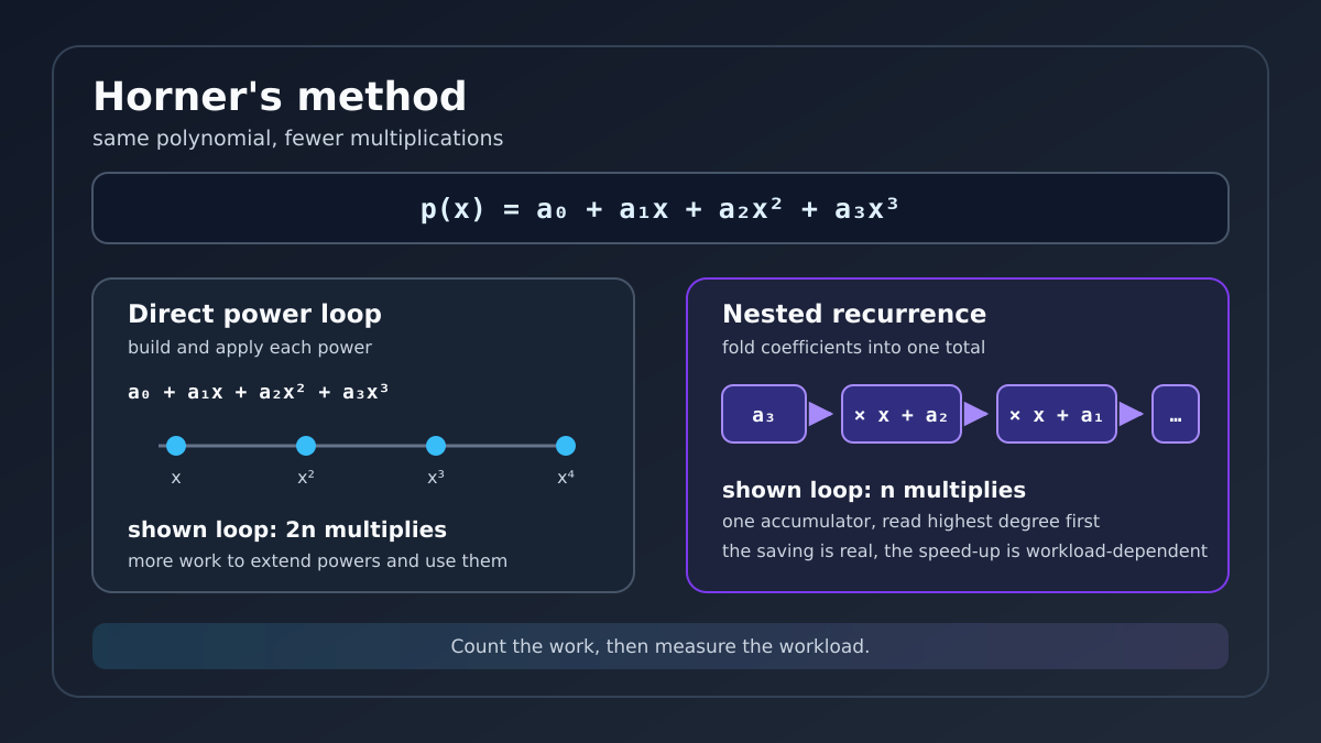
For a fixed value of x, the direct expression calculates powers such as x², x³ and x⁴, then multiplies each one by its coefficient. That is readable on paper. In a loop, it means doing a fresh multiplication to extend the power and another to apply the coefficient.
Horner’s method rewrites the same polynomial as a nest of multiply-and-add steps. The NIST recurrence processes each coefficient from the highest degree down and finishes with the polynomial value.[1]
The useful question is not whether the two formulas are mathematically equal. They are. The useful question is whether the saved work shows up in the Python program you are actually running.
The baseline: build each power as we go
The baseline below keeps its coefficients in ascending order: the first value is the constant term, followed by the coefficient of x, then x², and so on. It starts with the constant term, grows the next power with power *= x, and multiplies that power by the next coefficient.
For the stored implementation, that gives two multiplications per degree: one to apply the coefficient and one to update power. The final power update is unused, a deliberate consequence of keeping this baseline loop simple. The running total also needs one addition per degree.
The nested idea
Horner’s method starts at the highest-degree coefficient and folds coefficients into one accumulator:
p(x) = a₀ + x(a₁ + x(a₂ + ... + x aₙ))
Each pass does total = total * x + coefficient. For a degree n polynomial, the loop performs n multiplications and n additions. Its scalar state is small: the accumulator, the current coefficient and x. This exact Python implementation also creates tuple slices with coefficients[1:] and coefficients[:-1], so those temporary allocations grow with the degree. The scalar recurrence is constant-state, but the supplied code does not have constant allocation behaviour.
The order matters. With coefficients stored from the constant term upwards, Horner’s loop must read them backwards. If the coefficients arrive highest-first, the loop can use them directly. Treat coefficient order as part of the interface, not as a detail to tidy up later.
A complete comparison
Save this as horner_benchmark.py and run it with Python 3. The program checks the answers before timing anything, prints the arithmetic counts, and compares four polynomial degrees. It uses timeit.repeat, which runs several repetitions and lets us select the fastest sample. This script prints only the minimum from its seven samples, so the stored output does not expose the full timing vectors. Python’s documentation notes that other processes can make timings longer and recommends looking at the minimum rather than treating every slower sample as a change in Python’s speed. It also disables garbage collection by default during timed statements.[2]
The coefficient generator is deterministic and keeps the values bounded. The benchmark is therefore repeatable in its inputs, not magically identical in wall-clock time. CPU temperature, background work and the Python build still matter.
from __future__ import annotations

import math
import platform
import timeit


def direct_polynomial(coefficients: tuple[float, ...], x: float) -> float:
    """Evaluate a polynomial from constant term to highest term."""
    if not coefficients:
        raise ValueError("at least one coefficient is required")

    total = coefficients[0]
    power = x
    for coefficient in coefficients[1:]:
        total += coefficient * power
        power *= x
    return total


def horner_polynomial(coefficients: tuple[float, ...], x: float) -> float:
    """Evaluate a polynomial with Horner's nested recurrence."""
    if not coefficients:
        raise ValueError("at least one coefficient is required")

    total = coefficients[-1]
    for coefficient in reversed(coefficients[:-1]):
        total = total * x + coefficient
    return total


def make_coefficients(degree: int) -> tuple[float, ...]:
    """Create deterministic, bounded coefficients for the comparison."""
    return tuple((1.0 + (index % 9)) / (index + 1.0) for index in range(degree + 1))


def operation_counts(degree: int) -> tuple[tuple[int, int], tuple[int, int]]:
    """Return (multiplications, additions) for direct and Horner forms."""
    direct = (2 * degree, degree)
    horner = (degree, degree)
    return direct, horner


def benchmark(
    function, coefficients: tuple[float, ...], x: float, number: int
) -> tuple[float, list[float]]:
    timer = timeit.Timer(lambda: function(coefficients, x))
    samples = timer.repeat(repeat=7, number=number)
    return min(samples) / number, samples


def main() -> None:
    x = 0.75
    degrees_and_loops = ((8, 20_000), (32, 10_000), (128, 2_000), (512, 500))

    print(f"Python: {platform.python_version()}")
    print(f"Platform: {platform.platform()}")
    print(f"Machine: {platform.machine()}")
    print(f"Evaluation point: x={x}")
    print("Correctness checks:")

    for degree, _ in degrees_and_loops:
        coefficients = make_coefficients(degree)
        direct = direct_polynomial(coefficients, x)
        horner = horner_polynomial(coefficients, x)
        difference = abs(direct - horner)
        if not math.isclose(direct, horner, rel_tol=1e-12, abs_tol=1e-12):
            raise AssertionError(f"degree {degree}: results differ by {difference}")
        print(f"  degree={degree:3d}: value={horner:.12g}, absolute difference={difference:.3g}")

    print("\nOperation counts per evaluation:")
    print("degree | direct multiplications | Horner multiplications | additions")
    for degree, _ in degrees_and_loops:
        direct, horner = operation_counts(degree)
        print(f"{degree:6d} | {direct[0]:22d} | {horner[0]:21d} | {horner[1]:9d}")

    print("\nTiming, fastest of 7 repetitions:")
    print("degree | direct us | Horner us | direct/Horner")
    for degree, loops in degrees_and_loops:
        coefficients = make_coefficients(degree)
        direct_time, _ = benchmark(direct_polynomial, coefficients, x, loops)
        horner_time, _ = benchmark(horner_polynomial, coefficients, x, loops)
        print(
            f"{degree:6d} | {direct_time * 1e6:10.3f} | "
            f"{horner_time * 1e6:9.3f} | {direct_time / horner_time:13.2f}x"
        )


if __name__ == "__main__":
    main()
Python: 3.13.5
Platform: Linux-6.12.47+rpt-rpi-v8-aarch64-with-glibc2.41
Machine: aarch64
Evaluation point: x=0.75
Correctness checks:
  degree=  8: value=3.69966125488, absolute difference=0
  degree= 32: value=3.77079827967, absolute difference=4.44e-16
  degree=128: value=3.77084738382, absolute difference=4.44e-16
  degree=512: value=3.77084738382, absolute difference=4.44e-16

Operation counts per evaluation:
degree | direct multiplications | Horner multiplications | additions
     8 |                     16 |                     8 |         8
    32 |                     64 |                    32 |        32
   128 |                    256 |                   128 |       128
   512 |                   1024 |                   512 |       512

Timing, fastest of 7 repetitions:
degree | direct us | Horner us | direct/Horner
     8 |      1.468 |     1.338 |          1.10x
    32 |      4.282 |     3.495 |          1.23x
   128 |     16.226 |    12.286 |          1.32x
   512 |     61.551 |    45.534 |          1.35x
What the run measured
On the machine used for this draft, Horner’s method reduced the counted multiplications by half at every tested degree for the two stored functions. The timing ratio was measured separately for degrees 8, 32, 128 and 512, so the result is a comparison across those inputs rather than a promise about every polynomial or every Python installation.
The operation count is the cleaner result. The timings include Python function calls, loop overhead, float allocation, tuple slicing and the interpreter’s own work. They show the shape we care about: the stored baseline loop performs two multiplications per degree, including its final unused power update, while the stored Horner loop performs one. At small degrees, the difference may be too small to matter beside the rest of an application.
The script checks numerical agreement with math.isclose, not exact bit-for-bit identity. The two versions combine floating-point values in different orders, so tiny rounding differences are possible even though they implement the same polynomial. For ill-conditioned polynomials, changing the evaluation order can affect numerical error. NumPy’s documentation also warns that high-degree polynomial evaluation can be inaccurate because of rounding error.[4] Horner’s method is an efficient evaluation scheme, not a universal cure for a poorly scaled problem.
This example measures arithmetic work and wall-clock time, not memory. The two functions keep only a small scalar state during their loops, but the tuple slices described above allocate temporary tuples proportional to the degree. If allocation behaviour is the thing under investigation, Python’s tracemalloc module can report current and peak traced memory for a run.[3]
When it helps, and when it does not
Horner’s method is a good fit when the same polynomial is evaluated many times, the degree is high enough for arithmetic savings to matter, or the evaluation sits inside a tight loop. It is also a useful representation when a code review needs the number of arithmetic steps to be obvious.
It is less attractive when a library routine already evaluates the expression in a better specialised form, when the polynomial is tiny and clarity wins, or when many independent evaluations need parallel execution. A single Horner recurrence has a sequential dependency chain because each accumulator value depends on the previous one. As an engineering inference, grouping terms may expose more parallel work on suitable hardware, although that is a separate trade-off and can change rounding behaviour.
The theoretical count for the two functions in this article is simple: the stored direct loop performs 2n multiplications for degree n, while the stored Horner loop performs n. Those counts are not a universal tally for every direct implementation. The practical improvement is conditional. Measure the whole workload, include the cost of preparing coefficients and moving data, and keep the direct version as a correctness oracle during optimisation.
A small rule worth keeping
If a loop repeatedly computes powers of the same value, look for a recurrence before reaching for a faster machine. Sometimes the best optimisation is just to stop asking the machine to rediscover x × x in increasingly elaborate ways.
Sources
[1] NIST Digital Library of Mathematical Functions, Horner’s Scheme
[2] Python documentation, timeit
 read0nly